Drafting Batters in Fantasy Baseball, Part 1
My first season in fantasy baseball
I joined a fantasy baseball league for the first time this year, which may come as a shock to those of you who know that I love both baseball and data. I was in a fantasy basketball league a few years ago, but because I haven’t watched basketball seriously in about 15 years, these were two very unsatisfying seasons. I was hoping it would encourage me to watch more basketball, but instead I made zero moves, stubbornly refused to trade Kevin Durant, and effectively set my league fees on fire.

Unsurprisingly, this strategy did not help me win.
Finally, this year, a friend invited me to join his newly founded fantasy baseball league. The fees were a bit steep ($50), and I didn’t really make much progress in my prior fantasy leagues, but I decided to join up anyway. I actually watch baseball, and this seemed like a better incentive to learn how to play fantasy sports. So I signed up, with a vague sense that I was about to go down the rabbit hole.
There are a lot of parts to Fantasy Baseball, so I’m going to break this up into several posts. This series will focus on batters. I’m going to start this post with a brief introduction to Fantasy Baseball (geared toward those with little to no experience, and a limited understanding of baseball), this year’s draft strategy for batters, and reflections on the metrics I used. The second post will dive a little deeper into positional talent, and how that relates to the metrics I used. The third post will detail an alternate draft strategy, where I beat myself up about the drafting decisions I made. In the fourth post, I’ll look at the success of the team I drafted, and what I could have done differently. In each post, I included the R code I used to explore the player data and to develop a draft strategy, in case you are interested in implementing some of this analysis on your own. It’s also in my github repo.
I wrote this post because my initial search for fantasy baseball strategies returned many articles written for people with substantial prior fantasy sports experience. I wanted a reference for someone without significant experience in fantasy sports, that could be implemented by someone with a surface level understanding of baseball and minimal statistics knowledge. I decided to write the guide I wanted to read before this all began. Let’s begin.
What is fantasy baseball?
Fantasy leagues are made up of several teams competing against each other to win certain scoring categories. For those who have never played any fantasy sports, I’ll use my league as an example.
My league uses the following scoring categories:
| Batting | Pitching |
|---|---|
| Runs (R) | Strikeouts (SO) |
| Home Runs (HR) | Quality Starts (QS) |
| Runs Batted In (RBI) | Saves (SV) |
| Strikeouts (SO) | Earned Runs Average (ERA) |
| Stolen Bases (SB) | Walks, Hits per Inning Pitched (WHIP) |
| On Base Percentage Plus Slugging (OPS) | Strikeouts per Walk (SO_BB) |
If you aren’t super familiar with baseball and want to understand these scoring categories and any terminology that comes up, Fangraphs has a great glossary for offensive statistics and pitching statistics.
Each team in the league drafts players to create a roster, with the goal of winning as many scoring categories as possible. Each player’s real-life numbers contribute to the weekly matchup. For instance, if Mike Trout is on my fantasy team, and real-life Mike Trout hits three home runs that week, those three home runs count for my team.
Each week, my team plays against an opponent. If my team scores 20 runs that week, and my opponent’s team scores 18 runs that week, I win the Runs category for that week. If my team strikes out 10 times, and my opponent’s team strikes out 8 times, my opponent wins the Strikeouts category for that week (because striking out is bad). Categories won, lost, and tied are counted up each week. Throughout the 21 weeks of the fantasy season, I want to win as many categories as possible.
Before play begins, however, there is a league draft.
The draft
In the draft, each team takes turns drafting players to fill their available positions. For batting, there are a total of thirteen slots, comprising eight fielding positions (catcher, first base, second base, shortstop, third base, and left, center, and right field), plus two utility players (any position). There are also fourteen slots for pitchers. Seven slots are available for bench players, which can be divided up between batters and pitchers as you wish. I’ll discuss pitching in another post, but my drafted batters looked like this:
| Position | Name |
|---|---|
| Catcher (C) | Buster Posey (C) |
| First Base (1B) | Edwin Encarnacion (1B) |
| Second Base (2B) | Rougned Odor (2B) |
| Third Base (3B) | Mike Moustakas (3B) |
| Shortstop (SS) | Andrelton Simmons (SS) |
| Outfield (OF) | Mookie Betts (OF) |
| Outfield (OF) | Adam Jones (OF) |
| Outfield (OF) | Max Kepler (OF) |
| Utility (UTIL) | Brandon Crawford (SS) |
| Utility (UTIL) | Brandon Belt (1B) |
| Bench | Stephen Piscotty (OF) |
| Bench | Maikel Franco (3B) |
| Bench | Jose Peraza (SS) |
| Bench | Manuel Margot (OF) |
Drafted players are now on your team, but you can drop players who aren’t contributing, and add free agents who aren’t currently on a team throughout the season. You can also trade with other teams for players you want, up until the trade deadline.
The draft is important because this may be the only opportunity to pick up high performing players. Players like Mike Trout, or Mookie Betts, for instance, are unlikely to be dropped or traded, barring injury or disaster. It’s important to go into the draft with a strategy, or at least, some idea of how you want to select players. I’d previously spent maybe two hours preparing for my Fantasy Basketball drafts, so I thought this time, I’d devote an afternoon to it. This was not enough time, in hindsight.

How I prepared for the draft
I downloaded player projection data from Fangraphs. The projection is a prediction of how a player will perform, based on historical numbers. Each of the projection systems differs a bit, but the one I used was the ZIPS projection, because it was the first projection system I found on Fangraphs (I only had an afternoon, after all). I exported data from the site for each of the batting positions. I saved them to a folder called “data” in my R Project directory, renamed the files for readability, and combined all of the data for each position into one data frame called “batters”, with a variable called “position”. I also removed all other categories that I deemed irrelevant for making draft decisions. You can see this in the code below.
For reference, I’m loading in dplyr to facilitate data cleaning (and because I’m addicted to pipes), ggplot2 for easy visualizations, and purrr to simplify loading. I’m also loading in wesanderson to make my visualizations a little nicer to look at. I’ve written a function called load_data to minimize repetitive code. See the github repository for that code.
library(dplyr)
library(ggplot2)
library(purrr)
library(wesanderson)

source("../R/load_data.R")

pos_files <- c("../data/post1/depth_1B.csv", "../data/post1/depth_2b.csv", "../data/post1/depth_3b.csv", "../data/post1/depth_SS.csv", "../data/post1/depth_OF.csv", "../data/post1/depth_C.csv")
pos_names <- c("first_base", "second_base", "third_base", "short", "outfield", "catcher")
batters <- map2_df(pos_files, pos_names, load_data) %>%
  select(Name, Team, playerid, position, PA, R, HR, RBI, SB, OPS, SO, WAR)
My draft strategy
An afternoon is not enough time to learn about how to play fantasy baseball and come up with a cohesive, overarching draft strategy. Instead, I did a few quick calculations to empower me to make decisions about whom to draft in the moment, based on what players are available, what positions they play, which scoring categories are strengths for my team, and what gaps remain. To help inform timely draft decisions, I planned to create rank variables for each of the scoring categories, putting each player into quantiles for each category. Six scoring categories is an awful lot to synthesize in the two minutes given to select a player, so I needed to also rank some statistic that accounts for all six scoring categories. Based on my limited research, I decided to use WAR (Wins Above Replacement). WAR is often used as a summary statistic to characterize a player’s total contributions to their team.
How WAR is calculated differs by source. I got my projected WAR data from Fangraphs, which is calculated using a combination of offensive, defensive, and base running statistics. WAR was already part of the data I downloaded from Fangraphs, so I saved time not calculating a new statistic. However, all of my scoring categories are based on offensive statistics. WAR, while accounting for offensive statistics, also accounts for defense and base running, which are irrelevant to my scoring categories. Someone who has a high WAR may be excellent defensively, but may put up average offensive numbers. They may not help me win my scoring categories. I didn’t take this into account when preparing for my draft, but it ended up coming back to bite me later on.
WAR, what is it good for?
I looked at the distribution of projected WAR among all the players in the dataset, to understand how to split players into quantiles. I used a histogram to make sure the number of quantiles I wanted to split players into was large enough to capture the variance in WAR. If I split players up into too few quantiles, I might collapse exceptional players (WAR > 6) with reasonably good players (WAR = 3). If I split players into too many quantiles, I’ll end up with one player in each, which is not helpful for making comparisons.
ggplot(batters, aes(x=WAR)) +
  geom_histogram(bins = 50, fill = "#DD8D29") +
  theme_bw()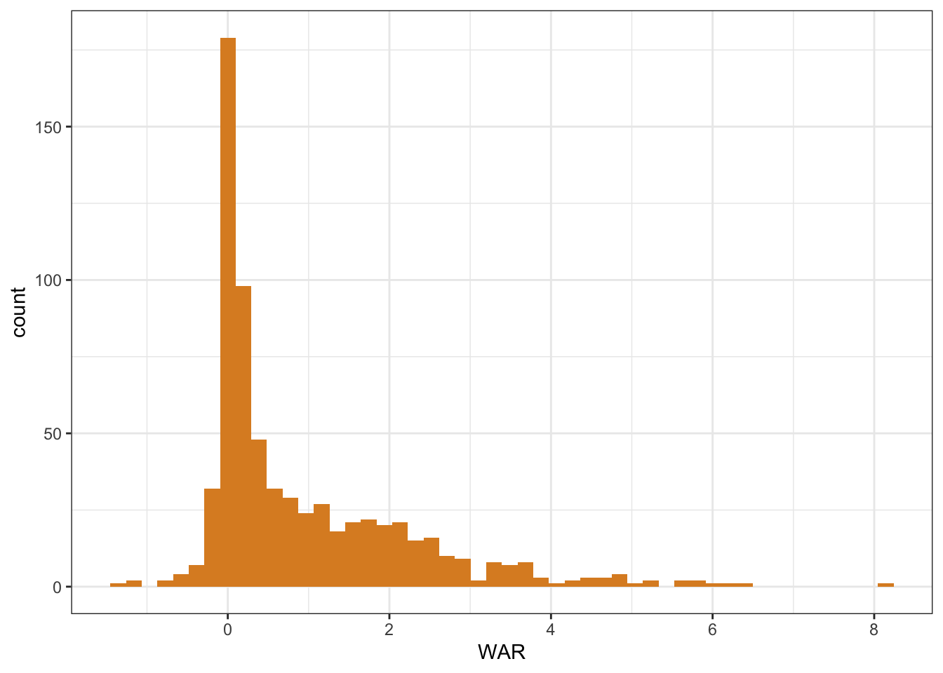
Based on the distribution, and the quantity that seemed reasonable to examine at a time, I decided to split batters up into quantiles of 50. My logic for this is that when choosing whom to draft, I’d be in good hands selecting any player in the top 2% of WAR. There were roughly 12-13 players in each quantile, which is enough to make comparisons across players. These players in the table below represent the top 2% in WAR.
batters$qt_WAR <- ntile(batters$WAR, 50)
batters %>%
  filter(qt_WAR == 50) %>%
  select(position, Name, WAR, SO, SB) %>%
  arrange(desc(WAR)) %>%
knitr::kable()| position | Name | WAR | SO | SB |
|---|---|---|---|---|
| outfield | Mike Trout | 8.2 | 131 | 22 |
| outfield | Giancarlo Stanton | 6.4 | 171 | 2 |
| third_base | Josh Donaldson | 6.2 | 134 | 4 |
| short | Carlos Correa | 6.1 | 121 | 8 |
| third_base | Kris Bryant | 5.9 | 147 | 9 |
| short | Francisco Lindor | 5.8 | 84 | 15 |
| outfield | Bryce Harper | 5.6 | 122 | 10 |
| outfield | Mookie Betts | 5.6 | 73 | 23 |
| third_base | Manny Machado | 5.3 | 105 | 8 |
| short | Corey Seager | 5.2 | 120 | 4 |
| third_base | Nolan Arenado | 5.0 | 101 | 3 |
| second_base | Jose Ramirez | 4.8 | 67 | 20 |
| third_base | Jose Ramirez | 4.8 | 67 | 20 |
Apologies to those on mobile, you may not be able to see all columns of these tables.
Jose Ramirez appears twice because he’s eligible to play two positions. This is helpful to know for drafting players, so I didn’t bother to clean this up.
I ended up selecting Mookie Betts in my first round, because in addition to a high WAR, he was projected to steal more bases (high SB), and strike out less often (low SO) than others in the top 2%. Nearly everyone else in this group was selected in the first round, so I needed to set my sights a little lower, the top 4%.
batters %>%
  filter(qt_WAR == 49) %>%
  select(position, Name, WAR, SO, SB) %>%
  arrange(desc(WAR)) %>%
knitr::kable()| position | Name | WAR | SO | SB |
|---|---|---|---|---|
| first_base | Joey Votto | 4.8 | 105 | 5 |
| second_base | Jose Altuve | 4.8 | 73 | 28 |
| first_base | Anthony Rizzo | 4.7 | 98 | 9 |
| third_base | Justin Turner | 4.6 | 84 | 6 |
| third_base | Anthony Rendon | 4.6 | 100 | 8 |
| outfield | George Springer | 4.5 | 137 | 9 |
| catcher | Buster Posey | 4.5 | 62 | 4 |
| outfield | Aaron Judge | 4.4 | 198 | 7 |
| first_base | Freddie Freeman | 4.3 | 134 | 8 |
| first_base | Paul Goldschmidt | 4.3 | 147 | 17 |
| outfield | Kevin Kiermaier | 4.1 | 134 | 21 |
| third_base | Kyle Seager | 3.9 | 106 | 3 |
| short | Andrelton Simmons | 3.8 | 64 | 13 |
A lot of these players had also been drafted, but of the ones remaining, I picked Buster Posey in the second round for his high WAR, and his low number of strikeouts relative to everyone else in his group. Andrelton Simmons was my fourth round pick for a similar reason, with more stolen bases.
Seems good so far, right?
As I mentioned above, WAR relies on more than just the scoring categories I care about. In fact, looking at Posey and Simmons, their projections for the scoring categories are low relative to other players with a similar WAR. They are on the lower end for scoring runs (R), hitting homeruns (HR), runs batted in (RBI), and getting on base/hitting for extra bases (OPS).
batters %>%
  filter(qt_WAR == 49) %>%
  select(position, Name, R, HR, RBI, SO, SB, OPS, WAR) %>%
knitr::kable()| position | Name | R | HR | RBI | SO | SB | OPS | WAR |
|---|---|---|---|---|---|---|---|---|
| first_base | Joey Votto | 95 | 28 | 92 | 105 | 5 | 0.952 | 4.8 |
| first_base | Freddie Freeman | 92 | 31 | 93 | 134 | 8 | 0.935 | 4.3 |
| first_base | Anthony Rizzo | 97 | 34 | 107 | 98 | 9 | 0.927 | 4.7 |
| first_base | Paul Goldschmidt | 101 | 31 | 103 | 147 | 17 | 0.927 | 4.3 |
| second_base | Jose Altuve | 94 | 20 | 82 | 73 | 28 | 0.859 | 4.8 |
| third_base | Justin Turner | 77 | 22 | 84 | 84 | 6 | 0.856 | 4.6 |
| third_base | Anthony Rendon | 85 | 22 | 86 | 100 | 8 | 0.849 | 4.6 |
| third_base | Kyle Seager | 79 | 28 | 92 | 106 | 3 | 0.816 | 3.9 |
| short | Andrelton Simmons | 70 | 11 | 67 | 64 | 13 | 0.710 | 3.8 |
| outfield | Aaron Judge | 99 | 41 | 106 | 198 | 7 | 0.901 | 4.4 |
| outfield | George Springer | 100 | 31 | 86 | 137 | 9 | 0.861 | 4.5 |
| outfield | Kevin Kiermaier | 76 | 19 | 62 | 134 | 21 | 0.743 | 4.1 |
| catcher | Buster Posey | 64 | 14 | 69 | 62 | 4 | 0.821 | 4.5 |
Picking these two in the second and fourth round, in hindsight, was not the best idea. In fact, it may not make sense to use WAR to differentiate between players in the early rounds because there is a high opportunity cost to missing out on strong offensive players that actually contribute to my scoring categories. Sorry, Buster.

WARning signs
I decided to look at how each of the scoring categories related to projected WAR. To do that, I standardized the scoring categories to simplify interpretation and visualization, since the range differs greatly across the scoring categories. Then, I plotted the standardized version against projected WAR.
source("../R/z_score.R")

ggplot(batters %>%
  mutate(
    R_z = z_score(R),
    HR_z = z_score(HR),
    RBI_z = z_score(RBI),
    OPS_z = z_score(OPS),
    SB_z = z_score(SB),
    SO_z = -z_score(SO)) %>%
  select(position, Name, Team, R_z, HR_z, RBI_z, SB_z, OPS_z, SO_z, WAR) %>%
  tidyr::gather(key = stat, value = value, R_z, HR_z, RBI_z, SB_z, OPS_z, SO_z),
  aes(x=WAR, y = value, colour = stat)) +
  geom_point() +
  facet_wrap(~stat, nrow = 3) +
  theme_bw() +
  scale_colour_manual(values = wes_palette("FantasticFox1", 6, type = "continuous")) +
  theme(legend.position="none")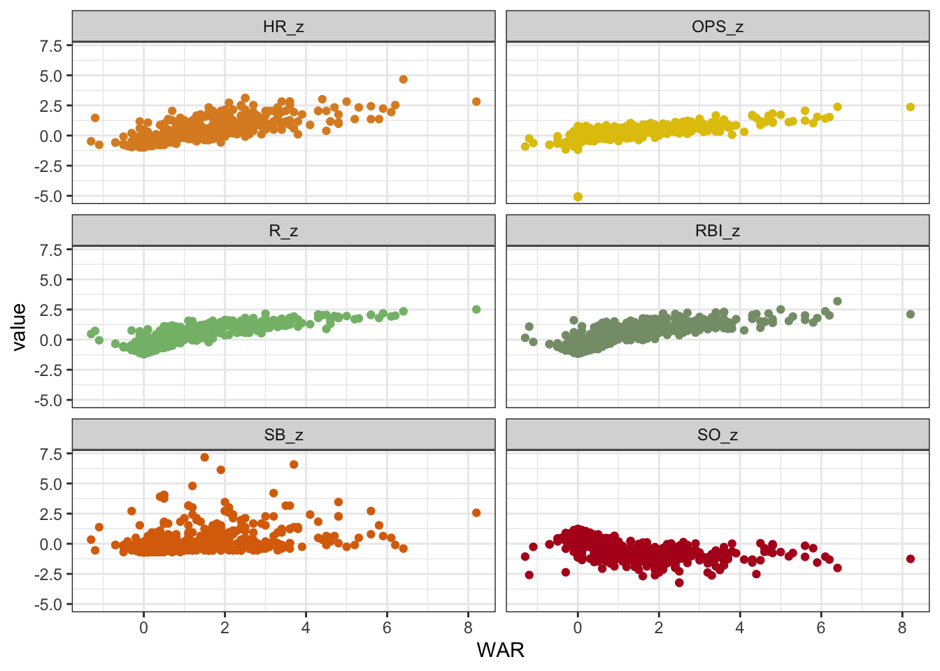
Looking at these plots, projected WAR seems to increase slightly with the first four scoring categories, but it doesn’t seem to increase with stolen bases (SB_z), or strikeouts (SO_z) at all.
WAR is not the answer (good god, y’all)
It looks like WAR isn’t great for identifying players that would help win my scoring categories, and it’s not at all related to stealing bases or striking out. I shouldn’t rely on this overall summary category to guide my decisions. Instead, perhaps it’d be more useful to rank players based on their projected performance for each scoring category. The performance in the scoring categories is ultimately what matters, and what will decide whether my team wins the matchup that week.
At this point in the draft, I changed strategies, and split players into quantiles by 50 again, and ranked each scoring category separately. This time, I filtered results to players who were in the top 4% of projections for runs, home runs, runs batted in, and on base plus slugging. I limited it to these four scoring categories because no player was in the top 4% for all six, and only Mike Trout was in the top 4% for these four categories plus base stealing.
While I’m sure it’s useful to know how great Mike Trout is, he was already picked up by some other team at this point. Nothing to see here.
So which players are the cream of the crop for my four scoring categories?
batters <- batters %>%
  mutate(qt_R = ntile(batters$R, 50),
         qt_HR = ntile(batters$HR, 50),
         qt_RBI = ntile(batters$RBI, 50),
         qt_OPS = ntile(batters$OPS, 50),
         qt_SO = ntile(desc(batters$SO), 50),
         qt_SB = ntile(batters$SB, 50))

batters %>%
  filter(qt_R > 48 & qt_HR > 48 & qt_RBI > 48 & qt_OPS > 48) %>%
  select(position, Name, R, HR, RBI, OPS, SO, SB) %>%
knitr::kable()| position | Name | R | HR | RBI | OPS | SO | SB |
|---|---|---|---|---|---|---|---|
| first_base | Anthony Rizzo | 97 | 34 | 107 | 0.927 | 98 | 9 |
| first_base | Rhys Hoskins | 92 | 36 | 111 | 0.877 | 140 | 5 |
| first_base | Edwin Encarnacion | 92 | 36 | 109 | 0.869 | 131 | 2 |
| third_base | Nolan Arenado | 97 | 39 | 118 | 0.937 | 101 | 3 |
| third_base | Josh Donaldson | 98 | 36 | 102 | 0.912 | 134 | 4 |
| outfield | Mike Trout | 114 | 39 | 105 | 1.027 | 131 | 22 |
| outfield | Giancarlo Stanton | 109 | 58 | 140 | 1.029 | 171 | 2 |
| outfield | Bryce Harper | 100 | 35 | 102 | 0.984 | 122 | 10 |
| outfield | Aaron Judge | 99 | 41 | 106 | 0.901 | 198 | 7 |
| outfield | Rhys Hoskins | 92 | 36 | 111 | 0.877 | 140 | 5 |
This group is in the top 4% of projections for runs, home runs, runs batted in, and OPS. This would have been a solid group to start with. I started seleting players based on this strategy and loosened the filtering criteria as we got further along in the draft. I also made sure to occasionally select players who were projected to have more stolen bases and fewer strikeouts. This strategy requires a lot of analysis in the moment, which can lead to a very stressful three hour draft.

In hindsight, I would have been better off spending more than an afternoon strategizing. I have regrets.
Up next
In the next part, I’ll explore positional talent as it relates to my draft decisions. Nevermind that I drafted Buster Posey in the second round, but should I have drafted ANY catcher in the second round? Would I have been better off drafting a player from some other position? Which positions are preferable to select from in the early rounds? This will all be covered in the next post. Stay tuned!